Machine Learning Exercise 1 - Linear Regression
This notebook covers a Python-based solution for the first programming exercise of the machine learning class on Coursera. Please refer to the exercise text for detailed descriptions and equations.
In this exercise we’ll implement simple linear regression using gradient descent and apply it to an example problem. We’ll also extend our implementation to handle multiple variables and apply it to a slightly more difficult example.
Linear regression with one variable
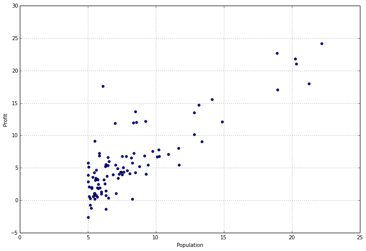
In the first part of the exercise, we’re tasked with implementing linear regression with one variable to predict profits for a food truck. Suppose you are the CEO of a restaurant franchise and are considering different cities for opening a new outlet. The chain already has trucks in various cities and you have data for profits and populations from the cities.
Let’s start by importing some libraries and examining the data.
import numpy as np
import pandas as pd
import matplotlib.pyplot as plt
%matplotlib inline
import os
path = os.getcwd() + '\data\ex1data1.txt'
data = pd.read_csv(path, header=None, names=['Population', 'Profit'])
data.head()
|
Population |
Profit |
| 0 |
6.1101 |
17.5920 |
| 1 |
5.5277 |
9.1302 |
| 2 |
8.5186 |
13.6620 |
| 3 |
7.0032 |
11.8540 |
| 4 |
5.8598 |
6.8233 |
|
Population |
Profit |
| count |
97.000000 |
97.000000 |
| mean |
8.159800 |
5.839135 |
| std |
3.869884 |
5.510262 |
| min |
5.026900 |
-2.680700 |
| 25% |
5.707700 |
1.986900 |
| 50% |
6.589400 |
4.562300 |
| 75% |
8.578100 |
7.046700 |
| max |
22.203000 |
24.147000 |
Let’s plot it to get a better idea of what the data looks like.
data.plot(kind='scatter', x='Population', y='Profit', figsize=(12,8))
<matplotlib.axes._subplots.AxesSubplot at 0xd140198>
Now let’s implement linear regression using gradient descent to minimize the cost function. The equations implemented in the following code samples are detailed in “ex1.pdf” in the “exercises” folder.
First we’ll create a function to compute the cost of a given solution (characterized by the parameters theta).
def computeCost(X, y, theta):
    inner = np.power(((X * theta.T) - y), 2)
    return np.sum(inner) / (2 * len(X))
Let’s add a column of ones to the training set so we can use a vectorized solution to computing the cost and gradients.
data.insert(0, 'Ones', 1)
Now let’s do some variable initialization.
# set X (training data) and y (target variable)
cols = data.shape[1]
X = data.iloc[:,0:cols-1]
y = data.iloc[:,cols-1:cols]
Let’s take a look to make sure X (training set) and y (target variable) look correct.
|
Ones |
Population |
| 0 |
1 |
6.1101 |
| 1 |
1 |
5.5277 |
| 2 |
1 |
8.5186 |
| 3 |
1 |
7.0032 |
| 4 |
1 |
5.8598 |
|
Profit |
| 0 |
17.5920 |
| 1 |
9.1302 |
| 2 |
13.6620 |
| 3 |
11.8540 |
| 4 |
6.8233 |
The cost function is expecting numpy matrices so we need to convert X and y before we can use them. We also need to initialize theta.
X = np.matrix(X.values)
y = np.matrix(y.values)
theta = np.matrix(np.array([0,0]))
Here’s what theta looks like.
Let’s take a quick look at the shape of our matrices.
X.shape, theta.shape, y.shape
((97L, 2L), (1L, 2L), (97L, 1L))
Now let’s compute the cost for our initial solution (0 values for theta).
So far so good. Now we need to define a function to perform gradient descent on the parameters theta using the update rules defined in the text.
def gradientDescent(X, y, theta, alpha, iters):
    temp = np.matrix(np.zeros(theta.shape))
    parameters = int(theta.ravel().shape[1])
    cost = np.zeros(iters)

    for i in range(iters):
        error = (X * theta.T) - y

        for j in range(parameters):
            term = np.multiply(error, X[:,j])
            temp[0,j] = theta[0,j] - ((alpha / len(X)) * np.sum(term))

        theta = temp
        cost[i] = computeCost(X, y, theta)

    return theta, cost
Initialize some additional variables - the learning rate alpha, and the number of iterations to perform.
alpha = 0.01
iters = 1000
Now let’s run the gradient descent algorithm to fit our parameters theta to the training set.
g, cost = gradientDescent(X, y, theta, alpha, iters)
g
matrix([[-3.24140214, 1.1272942 ]])
Finally we can compute the cost (error) of the trained model using our fitted parameters.
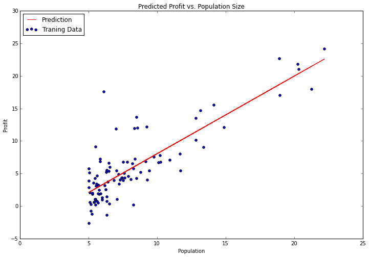
Now let’s plot the linear model along with the data to visually see how well it fits.
x = np.linspace(data.Population.min(), data.Population.max(), 100)
f = g[0, 0] + (g[0, 1] * x)

fig, ax = plt.subplots(figsize=(12,8))
ax.plot(x, f, 'r', label='Prediction')
ax.scatter(data.Population, data.Profit, label='Traning Data')
ax.legend(loc=2)
ax.set_xlabel('Population')
ax.set_ylabel('Profit')
ax.set_title('Predicted Profit vs. Population Size')
<matplotlib.text.Text at 0xd35a518>
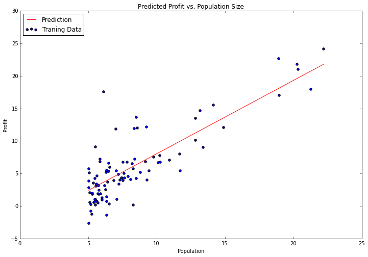
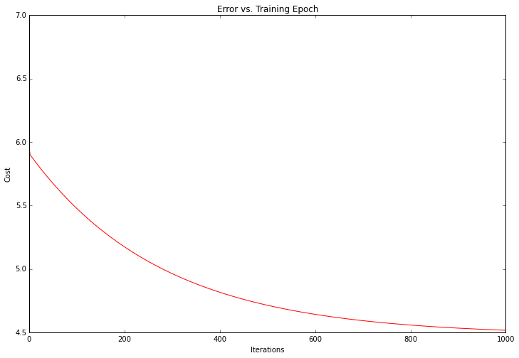
Looks pretty good! Since the gradient decent function also outputs a vector with the cost at each training iteration, we can plot that as well. Notice that the cost always decreases - this is an example of a convex optimization problem.
fig, ax = plt.subplots(figsize=(12,8))
ax.plot(np.arange(iters), cost, 'r')
ax.set_xlabel('Iterations')
ax.set_ylabel('Cost')
ax.set_title('Error vs. Training Epoch')
<matplotlib.text.Text at 0xd5bccc0>
Linear regression with multiple variables
Exercise 1 also included a housing price data set with 2 variables (size of the house in square feet and number of bedrooms) and a target (price of the house). Let’s use the techniques we already applied to analyze that data set as well.
path = os.getcwd() + '\data\ex1data2.txt'
data2 = pd.read_csv(path, header=None, names=['Size', 'Bedrooms', 'Price'])
data2.head()
|
Size |
Bedrooms |
Price |
| 0 |
2104 |
3 |
399900 |
| 1 |
1600 |
3 |
329900 |
| 2 |
2400 |
3 |
369000 |
| 3 |
1416 |
2 |
232000 |
| 4 |
3000 |
4 |
539900 |
For this task we add another pre-processing step - normalizing the features. This is very easy with pandas.
data2 = (data2 - data2.mean()) / data2.std()
data2.head()
|
Size |
Bedrooms |
Price |
| 0 |
0.130010 |
-0.223675 |
0.475747 |
| 1 |
-0.504190 |
-0.223675 |
-0.084074 |
| 2 |
0.502476 |
-0.223675 |
0.228626 |
| 3 |
-0.735723 |
-1.537767 |
-0.867025 |
| 4 |
1.257476 |
1.090417 |
1.595389 |
Now let’s repeat our pre-processing steps from part 1 and run the linear regression procedure on the new data set.
# add ones column
data2.insert(0, 'Ones', 1)

# set X (training data) and y (target variable)
cols = data2.shape[1]
X2 = data2.iloc[:,0:cols-1]
y2 = data2.iloc[:,cols-1:cols]

# convert to matrices and initialize theta
X2 = np.matrix(X2.values)
y2 = np.matrix(y2.values)
theta2 = np.matrix(np.array([0,0,0]))

# perform linear regression on the data set
g2, cost2 = gradientDescent(X2, y2, theta2, alpha, iters)

# get the cost (error) of the model
computeCost(X2, y2, g2)
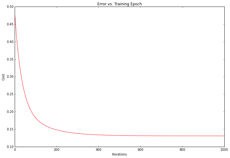
We can take a quick look at the training progess for this one as well.
fig, ax = plt.subplots(figsize=(12,8))
ax.plot(np.arange(iters), cost2, 'r')
ax.set_xlabel('Iterations')
ax.set_ylabel('Cost')
ax.set_title('Error vs. Training Epoch')
<matplotlib.text.Text at 0xd7bb240>
Instead of implementing these algorithms from scratch, we could also use scikit-learn’s linear regression function. Let’s apply scikit-learn’s linear regressio algorithm to the data from part 1 and see what it comes up with.
from sklearn import linear_model
model = linear_model.LinearRegression()
model.fit(X, y)
LinearRegression(copy_X=True, fit_intercept=True, normalize=False)
Here’s what the scikit-learn model’s predictions look like.
x = np.array(X[:, 1].A1)
f = model.predict(X).flatten()

fig, ax = plt.subplots(figsize=(12,8))
ax.plot(x, f, 'r', label='Prediction')
ax.scatter(data.Population, data.Profit, label='Traning Data')
ax.legend(loc=2)
ax.set_xlabel('Population')
ax.set_ylabel('Profit')
ax.set_title('Predicted Profit vs. Population Size')
<matplotlib.text.Text at 0xf258860>
That’s it! Thanks for reading. In Exercise 2 we’ll take a look at logistic regression for classification problems.